3D TRISO tutorial

TRISO (Tristructural Isotropic) fuel is an advanced type of nuclear fuel designed for high-temperature gas-cooled reactors. It consists of small spherical fuel kernels encapsulated in multiple layers of coatings. These layers provide a robust defense against the release of radioactive materials, even under extreme conditions, making TRISO fuel highly attractive for next-generation nuclear reactors due to its enhanced safety features and improved fuel performance.

Currently, OFFBEAT can perform 1D and 3D TRISO simulations. This page will introduce 3D TRISO simulations, including the mesh used in the simulation, boundary condition settings, OFFBEAT settings, control settings, etc.

In general, the difference between 3D TRISO simulation and 1D TRISO simulation is not much. The main difference lies in Boundary conditions and OFFBEAT setting. You can have a preliminary understanding of 3D TRISO simulations through this tutorial.

Mesh

For the mesh in 3D cases, this tutorial provides two ways to generate mesh, the first is through the provided script, the second is to use Coreform Cubit to generate.

1) Generate mesh using the provided script

OFFBEAT also provides another script to create an octant 3-D sphere. The script shares the similar input as the 1-D mesh script, but it requires three additional parameters. The script is located at ./offbeat/tools/sphereMaker_3D.

ratioOtype - The ratio of O-type mesh over the whole Kernel mesh.
ratio - The ratio of O-type mesh's edge length at X, Y, Z axis over its original radio.
hoopMesh - 2 times of this value will be used for the cell number along circumferential directions.

'ratioOtype':         0.7,
'ratio':              0.8,
'hoopMesh':           20,

Image title — TRISO 3 Dimensional Mesh generated by script

Note

For 3D mesh generated by theh script, only TRISO with all layers can be generated.

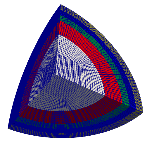
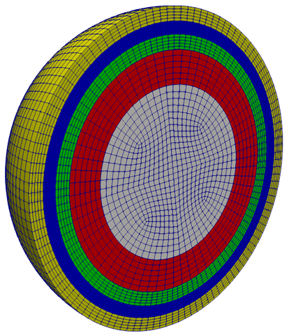
2) Generate mesh using the Coreform Cubit

In our current work, we used the Coreform Cubit to generate 3D mesh. This method allows us to use a coarse mesh for the Kernel and Buffer, and a finer mesh for the IPyC, SiC, and OPyC layers. For the use of this software, please refer to the official tutorial.

Boundary conditions

The TRISO simulation typically requires 2 initial fields, DD(or D) and T, to be provided at /0 folder, along with a uniform value gapGas at /0/uniform folder. The following part will give an example to show how it works in 3-D cases.

DD/D

DD represents the displacement increment. If the geometery you are building is a part of a TRISO particle (such as an octant or a quarter of a TRISO particle), you need to specify the symmetric surfaces as "symmetry". For example:

"bottom|top|front|back"
{
    type            symmetry;
}

The "bufferOuter" and "ipycInner" are usually coupled since they can have a contact between them. These settings are same as 1D cases:

"bufferOuter|ipycInner"
{
    type            gapContact;
    patchType       regionCoupledOFFBEAT;
    penaltyFactor   0.0;
    frictionCoefficient        0;
    relax           1.0;
    relaxInterfacePressure           0.1;
    traction        uniform (0 0 0);
    pressure        uniform 0.0;
    value           $internalField;
}

The "outer" surface is usually assigned a constant pressure. It is same as 1D cases:

outer
{
    type            tractionDisplacement;
    traction        uniform (0 0 0);
    pressure        uniform 0.1e6;
    value           uniform (0 0 0);
}

If you choose smallStrain instead of smallStrainIncrementalUpdated in mechanicsSolver, you need to set boundary conditions for D. D represents the displacement. The settings of D and DD are almost the same. The only difference is to change DD in FoamFile to D.

FoamFile
{
    version     2.0;
    format      ascii;
    class       volVectorField;
    object      D;
}

T

The input for the symmetric patches is the same as DD. Additionally, the "bufferOuter" and "ipycInner" patches are coupled using trisoGap to account for heat transfer between them.

bufferOuter
{
    type            trisoGap;
    patchType       regionCoupledOFFBEAT;
    kappa           k;
    coupled         true;
    roughness       uniform 1e-6;
    jumpDistance    uniform 0.0;
    value           $internalField;
    relax           1;
}

ipycInner
{
    type            trisoGap;
    patchType       regionCoupledOFFBEAT;
    kappa           k;
    coupled         true;
    roughness       uniform 1e-6;
    jumpDistance    uniform 0.0;
    value           $internalField;
    relax           1;
}

The "outer" is usually given a constant temperature.

outer
{
    type            fixedValue;
    value           uniform 1298;
}

gapGas

The gapGas represents the gas present between the bufferOuter and ipycInner layers, as well as inside the buffer. At the initial stage, massFractions and gasPressure are both set to 0 since there's no gap and no filling gas. gasPressureType is set to fromModel so that the quantity of these gas can be calculated by corresponding models. For more information about the model, users can refer to gapTRISO

massFractions
{
    Ar 0;
    He 0;
    Kr 0;
    Ne 0;
    Rn 0;
    Xe 0;
    CO 0;
};

gasPressureType                 fromModel;
gasPressure                     0;

OFFBEAT settings (solverDict)

The solverDict for TRISO is generally similar to every other OFFBEAT solverDict, except for several special points.

The mechanicsSolver usually use smallStrain in 3D cases.

timeDependentVhgr is usually used for volumetric heatsource and TRISO is typical type of gapGas but it also includes the compentence for CO production.

//Thermal and Mechanical solver selection:
thermalSolver           solidConduction;
mechanicsSolver         smallStrain; //(1)
neutronicsSolver        fromLatestTime;
elementTransport        fromLatestTime;

//Material and rhelogy treatment:
materialProperties      byZone;
rheology                byMaterial;

heatSource              timeDependentVhgr; //(2)
burnup                  fromPower;
fastFlux                timeDependentAxialProfile;
corrosion               fromLatestTime;
gapGas                  TRISO; //(3)
fgr                     SCIANTIX;

Compared to smallStrainIncrementalUpdated, smallStrain is more suitable for 3D TRISO simulation.
timeDependentVhgr is usually used for volumetric heatsource.
TRISO is a typical type of gapGas but it also includes the compentence for CO production.

As for 3-D case, it is recommended to use cellZone with the interfaceWeights and defaultWeights set to 1. Additionally, the sphericalStress can be enabled to generate the radial and hoop stress, strain and displacement fields.

mechanicsSolverOptions
{
    forceSummary        off;
    sphericalStress     on;
    multiMaterialCorrection
    {
        type                    cellZone;
        interfaceWeights        1;
        defaultWeights          1;
    }
}

Warning

For 3D single TRISO particle simulation, it is very important to set defaultWeights to 1, which will avoid errors in some numerical processes, especially the hoop stress distribution on the same surface in the SiC layer. That is, in theory, cells on the same surface should have the same hoop stress (due to the symmetry of TRISO particles), and when defaultWeights is less than 1, additional errors will be introduced, resulting in uneven stress distribution. However, for simulations of other non-single TRISO particles (such as a TRISO octant surrounded by a matrix), setting defaultWeights to 0.9 is acceptable, because the error in this case is not enough to have a significant impact on the calculation results.

The materials dictionary usually contains 4 blocks of materials to represent different regions of TRISO: Kernel(or UO2), Buffer, IPyC|OPyC (PyC) and SiC. Each of the materials has a corresponding class that defines all of its material properties and behaviors. Users are encouraged to check the use of different materials:

Here is a brief introduction to the materials dictionary:

Kernel

Kernel
  {
    material UO2;   // (1)
    densityModel            UO2Constant;
    heatCapacityModel       UO2MATPRO;  
    conductivityModel       UO2MATPRO;
    emissivityModel         constant;
    YoungModulusModel       constant;
    PoissonRatioModel       constant;
    thermalExpansionModel   constant;
    //
    densificationModel          none;
    swellingModel               none;
    relocationModel             none;

    emissivity emissivity [0 0 0 0 0]   0.0;
    E           E       [1 -1 -2 0 0]   2e8;
    nu          nu      [0 0 0 0 0]     0.345;
    alpha       alpha   [0 0 0 0 0]     10e-6;
    Tref        Tref    [0 0 0 1 0]     1298;

    enrichment                  0.167;
    rGrain                      5e-6;
    theoreticalDensity          10960;
    densityFraction             0.9863; //10810.0
    dishFraction                0.0;
    isotropicCracking           off;

    rheologyModel               elasticity;
  }

The material of the specified Kernel zone is UO2.

Buffer

  Buffer
  {
    material buffer;
    densityModel            constant;
    heatCapacityModel       constant;
    conductivityModel       constant;
    YoungModulusModel       constant;
    PoissonRatioModel       constant;
    thermalExpansionModel   constant;
    swellingModel           none;   //(1)
    emissivityModel         constant;

    rho         rho     [1 -3 0 0 0]    1010.0;
    Cp          Cp      [0 2 -2 -1 0]   720.0;
    k           k       [1 1 3 -1 0]    0.5;
    nu          nu      [0 0 0 0 0]     0.23;
    emissivity emissivity       [0 0 0 0 0]   1.0;
    E           E       [1 -1 -2 0 0]   2e8;
    alpha       alpha   [0 0 0 0 0]     5.5e-6;
    Tref        Tref    [ 0 0 0 1 0 ] 1298;

    rheologyModel               elasticity; //(2)
  }

The optional swellingModel also includes BufferPARFUME.
The optional creep model also includes PARFUMUEBufferCreepModel. In this example, we disabled the swelling and creep models of Buffer. But for more accurate simulation, these two models should be turned on.

IPyC/OPyC

"IPyC|OPyC"
    {
      material PyC;

      densityModel                constant;
      conductivityModel           constant;
      heatCapacityModel           constant;
      emissivityModel             constant;
      YoungModulusModel           constant;
      PoissonRatioModel           constant;
      swellingModel               PyCCorrelation;   //(1)
      radialCoefficients          (-1.43234e-1 2.62692e-1 -1.74247e-1 5.67549e-2 -8.36313e-3 4.52013e-4);
      tangentialCoefficients      (-3.24737e-2 9.07826e-3 -2.10029e-3 1.30457e-4 0.0 0.0);

      rho         rho     [1 -3 0 0 0]    1870.0;
      Cp          Cp      [0 2 -2 -1 0]   720.0;
      k           k       [1 1 3 -1 0]    4.0;
      emissivity emissivity [0 0 0 0 0]   1.0;
      E           E       [1 -1 -2 0 0]   3.96e10;
      nu          nu      [0 0 0 0 0]     0.33;
      alpha       alpha   [0 0 0 0 0]     5.5e-6;
      Tref        Tref    [0 0 0 1 0]     1298;

      rheologyModel misesPlasticCreep;
      rheologyModelOptions
      {
          plasticStrainVsYieldStress table
          (
              (0    1e60)
          );
          creepCoefficient         4.93e-4;
          poissonRationForCreep    0.4;
          relax 1;
          creepModel constantCreepPrincipalStress;  //(2)
          fluxConversionFactor       1.0;
      }
    }

The optional swellingModel also includes PyCPARFUME. Here we use the PyCCorrelation.
The optional creepModel also includes PARFUMUEPyCCreepModel. Here we use the constantCreepPrincipalStress.

SiC

SiC is set as a constant in the current simulations because its material properties are hardly affected by other conditions.

SiC
   {
    material constant;

    rho         rho     [1 -3 0 0 0]    3200.0;
    Cp          Cp      [0 2 -2 -1 0]   620.0;
    k           k       [1 1 3 -1 0]    13.9;
    emissivity emissivity [0 0 0 0 0]   0.0;
    E           E       [1 -1 -2 0 0]   3.7e11;
    nu          nu      [0 0 0 0 0]     0.13;
    alpha       alpha   [0 0 0 0 0]     4.9e-6;
    Tref        Tref    [0 0 0 1 0]     1298;

    rheologyModel               elasticity;
   }

Control settings (controlDict)

The controlDict file is a key configuration file in OFFBEAT. It manages global simulation settings, including runtime, time-stepping, data writing frequency, and enabling additional functions.

This is an example of controlDict in 3D TRISO cases. It is same as the controlDict in 1D cases.

//- Run options:
startFrom       latestTime; // (1)
startTime       0;          // (2)
stopAt          endTime;    // (3)
endTime         5e7;        // (4)
deltaT          1;          // (5)

//- Write options:
writeControl    timeStep;    // (6)
writeInterval   25;          // (7)
purgeWrite      0;           // (8)
writeFormat     ascii;       // (9)
writeCompression off;        // (10)
timeFormat      general;     // (11)
timePrecision   1;           // (12)
writePrecision  6;           // (13)

functions
{
    #includeFunc  probes;   // (14)
}

startFrom specifies where to start the simulation. Options include latestTime, startTime, and firstTime.
startTime is to specify the starting time of the simulation.
stopAt determines when the simulation should stop. Options include endTime and writeNow.
endTime specifies the physical time at which the simulation stops (600 days in this case).
deltaT defines the time step size for each simulation step.
writeControl specifies how often to write simulation data. Options include timeStep, runTime, adjustableRunTime, and clockTime.
writeInterval specifies the interval for writing simulation data, here every 25 time steps.
purgeWrite controls whether old data is deleted. 0 means no old data is deleted.
writeFormat specifies the format of the output data. Options include ascii and binary.
writeCompression determines whether output data is compressed. off means no compression is applied.
timeFormat defines the format for time outputs. Options include general, fixed, and scientific.
timePrecision specifies the number of decimal places for time outputs.
writePrecision specifies the number of decimal places for simulation data outputs.
#includeFunc probes activates the probes function to monitor variables at specified locations.

The Adjustable Time Step Options in OpenFOAM are used to dynamically control the size of the simulation time step during the runtime. This is particularly useful for simulations where certain physical or numerical conditions change over time, requiring smaller time steps in regions of rapid change (e.g., during steep gradients or high activity) and larger time steps when conditions are stable.

//- Adjustable time step options:
adjustableTimeStep true;           // (1)
maxDeltaT        2e5;              // (2)
minDeltaT         1;               // (3)
maxRelativeDeltaTIncrease 1e9;     // (4)
minRelativeDeltaTDecrease 1e9;     // (5)
maxRelativePowerIncrease  1e9;     // (6)
maxRelativePowerDecrease  1e9;     // (7)
maxBurnupIncrease 0.1;             // (8)
maxAverageCreep   1e-4;            // (9)
maxMaximumCreep   1e-4;            // (10)
maxFGR  1e-8;            // (11)

runTimeModifiable true;            // (12)

adjustableTimeStep allows the time step size to adjust dynamically based on simulation conditions.
maxDeltaT specifies the maximum allowable time step size. Here, it is set to 2e5 seconds.
minDeltaT specifies the minimum allowable time step size. Here, it is set to 1 second.
maxRelativeDeltaTIncrease sets the maximum relative increase in time step size between consecutive steps. Here, it is set to 1e9 (effectively unlimited).
minRelativeDeltaTDecrease sets the maximum relative decrease in time step size between consecutive steps. Here, it is also 1e9.
maxRelativePowerIncrease defines the maximum relative increase in power (or another monitored property) to permit a time step adjustment.
maxRelativePowerDecrease defines the maximum relative decrease in power (or another monitored property) to permit a time step adjustment.
maxBurnupIncrease limits the maximum allowable increase in burnup per time step. Here, it is capped at 0.1.
maxAverageCreep sets the maximum allowable average creep strain increment. Here, it is 1e-4.
maxMaximumCreep sets the maximum allowable creep strain increment at any location. Here, it is 1e-4.
maxFGR defines the maximum allowable fission gas release increment per time step. Here, it is 1e-8.
runTimeModifiable allows the simulation runtime settings (such as controlDict) to be modified during the simulation.

Probes/functions

The probe function in OFFBEAT is a post-processing utility that allows users to monitor and extract simulation data at specific points within the computational domain. The file is stored in /system. This data can include variables like stress, strain, temperature, or any other field of interest. Here is an example:

FoamFile
{
    version     2.0;
    format      ascii;
    class       dictionary;
    location    "system";
    object      probes;
}
// * * * * * * * * * * * * * * * * * * * * * * * * * * * * * * * * * * * * * //
points
(
    (387e-6 0.0 0.0) //(1)
);

fields  (sigma); //(2)

#includeEtc "caseDicts/postProcessing/probes/probes.cfg" //(3)

points: Specifies the locations in the domain where data will be probed. Here, a single point is defined at (387e-6 0.0 0.0) in Cartesian coordinates (x, y, z). This represents a location in the domain where probes will extract data.
fields: Specifies the fields (variables) to monitor at the defined probe points. Here, sigma is the field being monitored. It could represent stress, surface tension, or any scalar/tensor field defined in the simulation.
#includeEtc: Includes external configuration files to extend or modify the behavior of this dictionary.

Commands to run in order

The Allrun file automates the setup and execution of an 3D TRISO case. Each step performs a critical part of the simulation workflow, ensuring the case is prepared and executed correctly without manual intervention. Here is an example and explanation of Allrun file

#!/bin/sh                              // (1)
# Run from this directory
cd "${0%/*}" || exit 1                 // (2)

# Source tutorial run functions
. "$WM_PROJECT_DIR/bin/tools/RunFunctions" // (3)

runApplication -o blockMesh            // (4)
runApplication -o changeDictionary     // (5)
runApplication -o offbeat              // (6)

#!/bin/sh: This specifies the script interpreter as the shell (sh). It ensures the script runs in a compatible shell environment.
cd "${0%/*}" || exit 1: Changes the working directory to the directory containing the script itself. ${0%/*} extracts the directory path of the script. || exit 1 ensures the script exits with an error code (1) if changing the directory fails.
. "$WM_PROJECT_DIR/bin/tools/RunFunctions": Sources the RunFunctions script from the OpenFOAM installation directory. $WM_PROJECT_DIR is an environment variable pointing to the root directory of the OpenFOAM installation. RunFunctions contains predefined shell functions (like runApplication) that simplify running applications in OpenFOAM.
runApplication -o blockMesh: Executes the blockMesh utility to generate the computational mesh based on the blockMeshDict file. -o: Ensures any existing output from the command is overwritten.
runApplication -o changeDictionary: Executes the changeDictionary utility to update the case dictionary files with the specified modifications (e.g., boundary conditions, initial fields).
runApplication -o offbeat: Executes the offbeat solver.

The Allclean script is used to clean up all files and directories generated during a simulation run. It ensures the case directory is reset to its original state, ready for a new simulation run. This is an example of Allclean.

#!/bin/bash                               
cd ${0%/*} || exit 1                      

foamListTimes -rm                         // (1)
rm constant/polyMesh -rf                  // (2)
rm -f ./0/cellToRegion                    // (3)
rm -rf postProcessing                     // (4)
rm -rf Frames                             // (5)
rm -f log*                                // (6)
rm -f results*                            // (7)
rm -f *.png                               // (8)
rm -f *.OpenFOAM                          // (9)
rm -f *.foam                              // (10)
rm -f input_check.txt                     // (11)

foamListTimes -rm: Removes all time directories (folders corresponding to simulation time steps) generated by OpenFOAM. This is achieved using the foamListTimes utility with the -rm option.
rm constant/polyMesh -rf: Deletes the mesh directory located at constant/polyMesh recursively and forcibly.
rm -f ./0/cellToRegion: Removes the cellToRegion file in the 0 directory, which may store region-specific information. The -f option suppresses errors if the file doesn't exist.
rm -rf postProcessing: Deletes the postProcessing directory recursively. This directory contains post-processing results (e.g., sampled data or probes).
rm -rf Frames: Deletes the Frames directory recursively. This is often used to store image sequences or animations created during the simulation.
rm -f log*: Deletes all log files generated during the simulation, including files starting with log (e.g., log.blockMesh, log.foam).
rm -f results*: Deletes any files starting with results (e.g., result summaries or processed outputs).
rm -f *.png: Deletes all PNG image files in the current directory.
rm -f *.OpenFOAM: Deletes files with the .OpenFOAM extension, which may be used for visualization purposes.
rm -f *.foam: Deletes files with the .foam extension, commonly used to open cases in Paraview for visualization.
rm -f input_check.txt: Deletes the input_check.txt file, which may contain validation or diagnostic information.

Results

The examples in this tutorial are based on case 13 of IAEA CPR-6. If your settings are correct, running this case, you should get the following results: